Social Media Content And Beverages 🥤
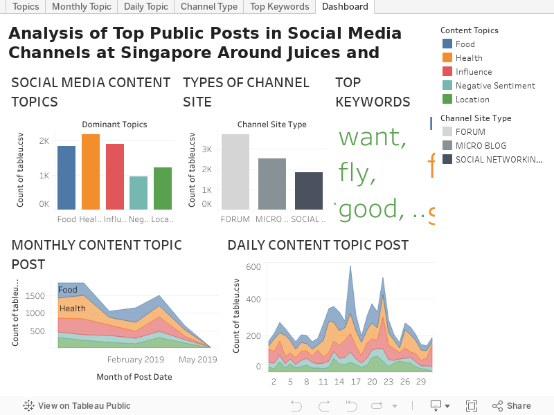
Analysis Of Top Public Posts In Social Media Channels At Singapore Around Juices And Beverages

⬛ Introduction
◼ There is an enormous amount of data being created on the internet every second — posts, comments, photos, and videos. These are types of data. But in this case, we are going to focus on Text, specifically about juices and beverages in social media channels in Singapore.
◼ All social media contents are based on written words — tweets, Facebook posts, comments, online reviews, and so on. Being a social media marketer, a Facebook group/profile moderator, or trying to promote your business on social media requires you to know how your audience reacts to the content you are uploading. One way is to read it all, what people feel towards juices and beverages, divide them into similar topic groups, calculate statistics.
⬛ What Makes Social Media Content So Unique?
◼ Before jumping to the analyses, it is really important to understand why social media texts are so unique:
✔️ Posts and comments are short. They mostly contain one simple sentence or even single word or expression. This gives us a limited amount of information to obtain just from one post.
✔️ Emojis and smiley faces — used almost exclusively on social media. They give additional details about the author’s emotions and context.
✔️ Slang phrases which make posts resemble spoken language rather than written. It makes statements appear more casual.
◼ These features make social media a whole different source of information and demand special attention while running an analysis using machine learning. In contrast, most open-source machine learning solutions are based on long, formal text, like Wikipedia articles and other website posts. As a result, these models perform badly on social media data, because they don’t understand additional forms of expression included.
⬛ Topic Modeling For Social Media Content
◼ Machine learning for text analysis is a vast field with lots of different model types that can gain insight into the data. But in this case, Topic Modeling will be more suitable in this analysis
◼ It can find topics which are patterns hidden within the data on its own without supervision and help — which makes it an unsupervised machine learning method. This means that it is easy to build a model for each individual problem.

◼ There are lots of different algorithms that can be used for this task, but the most common and widely used is LDA (Latent Dirichlet Allocation). It’s based on word frequencies and topics distribution in texts. To put it simply, this method counts words in a given data set and groups them based on their co-occurrence into topics. Then the percentage distribution of topics in each document is calculated.
◼ As a result this method assumes that each text is a mixture of topics which works great with long documents where every paragraph relates to a different matter.


🔔 Importing Modules
In [ ]:
# Importing modules
import pandas as pd
import os
os.chdir('..')

import numpy as np
import re, nltk, spacy, gensim

import logging
import warnings
warnings.filterwarnings('ignore')

from gensim.models.coherencemodel import CoherenceModel
from gensim.models.ldamodel import LdaModel
from gensim.corpora.dictionary import Dictionary
from numpy import array
In [ ]:
# Store dataset in a Pandas Dataframe
df = pd.read_csv('/content/social.csv')
In [ ]:
# Show the Title and Content column
df[['Title', 'Content']]
Out[ ]:
🔔 We can observed that we have 13 features and 8,072 rows of data but in this task we're just going to focus in getting juicy insights in social media's title and content column. And breakdown the data to make it more understandable to analysts so that they can decipher what are people saying around Juices & Beverages. 🍹
In [ ]:
# Check data dimension
df.shape
Out[ ]:
In [ ]:
# Check for missing values
df.isnull().mean()
Out[ ]:
🔔 In this part, we are going to clean and remove unnecessary characters that offers no value in generating insights and in order to process these data as well into the machine learning model.
1️⃣ Remove the punctuations.
2️⃣ Convert the contents to lowercase.
❌ Punctuations = '[,@#.!"#$%&()*+,-./:;<=>?@[\]^_`{|}~!?]',
In [ ]:
# Import regular expression library
import re

# Remove punctuation
df['Content'] = df['Content'].map(lambda x: re.sub('[,@#\.!"#$%&\'()*+,-./:;<=>?@[\\]^_`{|}~!?]','', x))

# Convert the contents to lowercase
df['Content'] = df['Content'].map(lambda x: x.lower())

# Print out the first rows of papers
df['Content'].head()
Out[ ]:
☁️ WorldCloud for Title
In [ ]:
# Import the wordcloud library
from wordcloud import WordCloud

# Join the different titles together.
long_string = ','.join(list(df['Title'].values))

# Generate the word cloud
wordcloud = WordCloud(background_color = 'white',
                      max_words = 500,
                      contour_width = 3,
                      contour_color = 'steelblue',
                      collocations = False, width=1000, height=400).generate(long_string)

# Visualize the word cloud
wordcloud.to_image()
Out[ ]:

🔔 You can see in the picture above the Title word cloud. The most dominant words are juice, orange, carrot, people, singapore, fresh, taste, share environment, inside, drink, fruits, vending, machine, clean, stay, away, shopping, Lot, everyone, etc
🔔 So it’s probably a topic about Food and Places. 🍔🥤

🔔 We can tell us a story that "People in Singapore likes Clean and Fresh Fruit Juices with a flavor of Orange and Carrot combination (probably taste good!) while Staying Inside in a Shared Enviroment with Everyone even if they're far Away from their Lot! or they can just grab a Drink in Vending Machine instead." Ha! 😎
☁️ WorldCloud For Content
In [ ]:
# Join the different processed Content together.
long_string = ','.join(list(df['Content'].values))

# Generate the word cloud
wordcloud2 = WordCloud(background_color = 'white',
                      max_words = 200,
                      contour_width = 3,
                      contour_color = 'steelblue',
                      collocations = False, width=1000, height=400).generate(long_string)

# Visualize the word cloud
wordcloud2.to_image()
Out[ ]:

🔔 For the Content Word cloud, it can be observed that the dominant words are somehow similar to the title word cloud. The topic is pretty much about food and drinks as well. Possible story with this is that "People likes to eat fresh and healthy food that has less content of sugar because they're thinking about their health?" 😃
⬛ Prepare Data For Topic Modelling
In [ ]:
# Set timer in processing
%%time

# Import libraries
import gensim
from gensim.utils import simple_preprocess

# Split sentences into words
def sent_to_words (sentences):
  for sentence in sentences:
    yield(gensim.utils.simple_preprocess(str(sentence), deacc = True))
data = df.Content.values.tolist()
data_words = list(sent_to_words(data))

# Check the data
print(data_words[:1])
In [ ]:
# Build the bigram and trigram models # higher threshold fewer phrases.
bigram = gensim.models.Phrases(data_words, min_count = 5, threshold = 100)
trigram = gensim.models.Phrases(bigram[data_words], threshold = 100)

# Faster way to get a sentence formatted as a bigram or trigram
bigram_mod = gensim.models.phrases.Phraser (bigram)
trigram_mod = gensim.models.phrases.Phraser (trigram)
In [ ]:
# NLTK Stop words
import nltk
nltk.download('stopwords')
from nltk.corpus import stopwords
stop_words = stopwords.words('english')
# stop_words.extend(['data', 'development', 'result', 'analysis', 'model'])

# Define functions for stopwords, bigrams, trigrams and lemmatization
def remove_stopwords(texts):
    return [[word for word in simple_preprocess(str(doc)) if word not in stop_words] for doc in texts]
def make_bigrams(texts):
    return [bigram_mod[doc] for doc in texts]
def make_trigrams(texts):
    return [trigram_mod[bigram_mod[doc]] for doc in texts]

# Lemmatization function
def lemmatization(texts, allowed_postags=['NOUN', 'ADJ', 'VERB', 'ADV']):
    """https://spacy.io/api/annotation"""
    texts_out = []
    for sent in texts:
      doc = nlp(" ".join(sent))
      texts_out.append([token.lemma_ for token in doc if token.pos_ in allowed_postags])
    return texts_out
In [ ]:
# Import spacy library
import spacy

# Remove Stop Words
data_words_nostops = remove_stopwords(data_words)

# Form Bigrams
data_words_bigrams = make_bigrams(data_words_nostops)

# Initialize spacy 'en' model, keeping only tagger component (for efficiency)
nlp = spacy.load('en_core_web_sm', disable = ['parser', 'ner'])

# Lemmatize keeping only noun, adj, vb, adv
data_lemmatized = lemmatization(data_words_bigrams, allowed_postags = ['NOUN', 'ADJ', 'VERB', 'ADV'])

# Check data
print(data_lemmatized[:1])
In [ ]:
# Import library
import gensim.corpora as corpora

# Create Dictionary
id2word = corpora.Dictionary(data_lemmatized)

# Create Corpus
texts = data_lemmatized

# Term Document Frequency
corpus = [id2word.doc2bow(text) for text in texts]

# View data
print(corpus[:2])
⬛ Build Topic Model

🔔 Statistical model for discovering the abstract "topics" that occur in a collection of documents. This will help us in text-mining to extract hidden semantic structures in a corpus. In order to find the optimal number of topics. We need to build many LDA models with different values of the number of topics (k) and pick the one that gives the highest coherence value.
🔔 Choosing a ‘k’ that marks the end of a rapid growth of topic coherence usually offers meaningful and interpretable topics. Picking an even higher value can sometimes provide more granular sub-topics. If we see the same keywords being repeated in multiple topics, it’s probably a sign that the ‘k’ is too large.
In [ ]:
# Build LDA model
lda_model = gensim.models.ldamodel.LdaModel(corpus = corpus,
                                            id2word = id2word,
                                            num_topics = 5,
                                            random_state = 123, # For reproducibility
                                            chunksize = 100,
                                            passes = 10,
                                            alpha = 0.01,
                                            eta = 'auto',
                                            iterations = 400,
                                            per_word_topics = True)

🔔 We can now observed keywords in the five topics at the output below.
🔔 This somehow gave us an idea about what could be a good label for each topics. LDA is an unsupervised learning so it is really up to human knowledge to determine what would be a suitable label for each topic.
💭 Topic 0 contains keywords such as 'power', 'big' and 'add'. Is this about Measurement?
💭 Topic 1 contains keywords such as 'juice', 'eat' and 'drink'. Is this about Food & Drinks?
💭 Topic 2 contains keywords such as 'say', 'think' and 'help'. Is this about Expression?
💭 Topic 3 contains keywords such as 'health', 'calorie', 'fat'. Is this about Health?
💭 Topic 4 contains keywords such as 'influencer', 'work' and 'daily'. Is this about Influence?
🔔 Don't worry, this will be further visualize later on 👍
In [ ]:
# Import library
from pprint import pprint

# Print the Keyword in the 5 topics
pprint(lda_model.print_topics())

# Transform corpus
doc_lda = lda_model[corpus]
⬛ Evaluation of Topic Model
🔔 LDA is an unsupervised technique, meaning that we don’t know prior to running the model how many topics exits in our corpus. We can use LDA visualization tool pyLDAvis, tried a few numbers of topics and compared the results.
🔔 Topic coherence is one of the main techniques used to estimate the number of topics and also a good way to compare difference topic models based on their human-interpretability.
🔔 We will use both UMass and c_v measure to see the coherence score of our LDA model because it capture the optimal number of topics by giving the interpretability of these topics a number called coherence score.
⬛ Coherence Score
✔ Perplexity = a measure of how good the model is. Lower value is preferred.
✔ C_v = Measure is based on a sliding window, one-set segmentation of the top words and an indirect confirmation measure that uses normalized pointwise mutual information (NPMI) and the cosine similarity
✔ umass = Based on document cooccurrence counts, a one-preceding segmentation and a logarithmic conditional probability as confirmation measure
In [ ]:
# Import library
from gensim.models import CoherenceModel

# Compute Perplexity
print('\nPerplexity: ', lda_model.log_perplexity(corpus) )

# Compute Coherence Score
coherence_model_lda = CoherenceModel (model = lda_model, texts = data_lemmatized, dictionary = id2word, coherence = 'c_v')
coherence_lda = coherence_model_lda.get_coherence()
print('\nCoherence Score: c_v ', coherence_lda)

# Compute Coherence Score using UMass
coherence_model_lda = CoherenceModel (model = lda_model, texts = data_lemmatized, dictionary = id2word, coherence = 'u_mass')
coherence_lda = coherence_model_lda.get_coherence()
print('\nCoherence Score u_mass: ', coherence_lda)
In [ ]:
# Intall Library
!pip install -U pyLDAvis

# Import library
import pyLDAvis.gensim
In [ ]:
# Visualize the topics
vis = pyLDAvis.gensim.prepare(lda_model, corpus, id2word)

# Show this in notebook
pyLDAvis.enable_notebook()

# Show visualization
vis
Out[ ]:
⬛ Interpretation
◼ Latent topics can then be found by searching for groups of words that frequently occur together in documents across the corpus Documents with similar topics use similar group of words.
◼ The distance between each topic bubble represent how semantic different they are. The farther they are, the better because it leads to a unique topic. A good model has to have distinct topics. It means no overlapping in bubbles.
◼ Finally, Everyone can create insights about in a particular aspect but - is that insight near in solving the actual problem? This is actually depends more on domain knowledge of an expert to fully analyze a particular field to determine the underlying concepts of each topic bubble.
⬛ Observation
⚫ Topic 1 - Food
This topic contains keywords such as food, sugar, juice, eat and drink.
⚫ Topic 2 - Health
This topic contains keywords such fat, health, calorie, body and vegetables.
⚫ Topic 3 - Influence
This topic contains keywords such influencers, chinese, industry, change and learn.
⚫ Topic 4 - Negative Sentiment
This topic contains keywords such remove, complain, toxic_enviroment, quit and problem.
⚫ Topic 5 - Location
This topic contains keywords such market, apartment, move, leave and big.
⬛ Conclusion
🔴 It can be observed the Food and Negative sentiment topic bubble overlapped in large size. It can be concluded that there is a huge negative feedbacks toward to food.
🔴 It can also observed that Health and Influence topic bubble overlapped a little bit. It means these two topics are somehow relatable to each other.
🔴 Topic 5 which is the Location Topic bubble are very far from the other topic bubbles. Location are greatly irrelevant to Food, Health, Influence and Negative sentiment.
In [ ]:
# Store content column
tc = df[['Content']]

# Get the probabilities being part of a certain topic
all_topics = lda_model.get_document_topics(doc_lda, minimum_probability = 0.0)
all_topics_csr = gensim.matutils.corpus2csc(all_topics)
all_topics_numpy = all_topics_csr.T.toarray()
all_topics_df = pd.DataFrame(all_topics_numpy)

# Content and topic probalities
result = pd.concat([tc, all_topics_df], axis = 1, sort = False)

# Check data columns
result.columns
Out[ ]:
In [ ]:
# Rename columns
result.columns = ['Content', 'Food', 'Health', 'Influence', 'Negative Sentiment', 'Location']

# Check data
result.head(10)
Out[ ]:
In [ ]:
# Function below nicely aggregates this information in a presentable table.
def format_topics_sentences(ldamodel=lda_model, corpus=corpus, texts=data):

    # Init output
    sent_topics_df = pd.DataFrame()

    # Get main topic in each document
    for i, row in enumerate(ldamodel[corpus]):
        row = sorted(row, key=lambda x: (x[1]), reverse=True)

        # Get the Dominant topic, Perc Contribution and Keywords for each document
        for j, (topic_num, prop_topic) in enumerate(row):
            if j == 0:  # => dominant topic
                wp = ldamodel.show_topic(topic_num)
                topic_keywords = ", ".join([word for word, prop in wp])
                sent_topics_df = sent_topics_df.append(pd.Series([int(topic_num), round(prop_topic,4), topic_keywords]), ignore_index=True)
            else:
                break
    sent_topics_df.columns = ['Dominant_Topic', 'Perc_Contribution', 'Topic_Keywords']

    # Add original text to the end of the output
    contents = pd.Series(texts)
    sent_topics_df = pd.concat([sent_topics_df, contents], axis=1)
    return(sent_topics_df)


df_topic_sents_keywords = format_topics_sentences(ldamodel=lda_model, corpus=corpus, texts=data)

# Format
df_dominant_topic = df_topic_sents_keywords.reset_index()
df_dominant_topic.columns = ['Document_No', 'Dominant_Topic', 'Topic_Perc_Contrib', 'Keywords', 'Text']

# Show
df_dominant_topic.head(10)
Out[ ]:

◼ Topic Correlations
In [ ]:
# Install library
!pip install heatmapz

# Import libraries
import pandas as pd
import numpy as np
import matplotlib.pyplot as plt
import seaborn as sns

# Show correlation in the features by using heatmap
from heatmap import corrplot
plt.figure(figsize=(12, 8))
corrplot(result.corr(), size_scale=300)

🔔 For some reason, the Influence Topic and Negative Sentiment Topic has a quite high negative correlation to each other in terms of their probabilities of being part in a certain topic class. While Influence Topic and Health Topic still shows a little correlation with each other and others with no correlation at all. We shoud also remember that correlation doesn't mean causation.
◼ Topic Frequency
In [ ]:
# Plot the number of Topic in dataset
plt.figure(figsize = (8, 8))
sns.countplot(y = "Dominant_Topic", data = df_dominant_topic)
plt.show()

🔔 We can observe the numbers of each topic class. A lot of people are really interested in Food Topic followed by Health Topic and then Influence Topic. This is a very valuable insights for the marketing team or business professionals - that it is highly recommended to focus their marketing campaign that relates to people's interest. In this case, Food and Fitness.
🔔 It can also be observed that most of the people active in social media are conscious about their diet, and most probably it is because of the Influencers that are fit, they're setting a standard of fitness through social media that could inspired other people to stay fit as well.
◼ Top Influential Channels
In [ ]:
# Channel column
channel_name = df['Channel Name']

# Get the channel value counts
unique, counts = np.unique(channel_name, return_counts = True)

# Channel counts
channel_counts = dict(zip(unique, counts))

# Transform into dataframe
channel_freq = pd.DataFrame(list(channel_counts.items()),columns = ['Channel_Name','Channel_Count'])

# Sort dataframe according to frequency
channel_freq = channel_freq.sort_values(by=['Channel_Count'], ascending = False )

# Add Post Type according to their respective indices
channel_freq['Post_type'] = df['Post Type']

# Add channel Type according to their respective indices
channel_freq['Channel_Type'] = df['Channel Site Type']

# Re-arrange columns
channel_freq = channel_freq[['Channel_Count', 'Channel_Name', 'Channel_Type', 'Post_type']]

# Check top infulential channels
channel_freq.head(10)
Out[ ]:
🔔 We can see here that Twitter channel has the highest influence in social media followed by HardwareZone Forum channel and then SG Talk channel. Comparing these top 3 channels to other channels, there's a huge gap in terms of numbers of content created by the users. We can also see that Microblogs has the highest frequency in channel type, while Comments as type of post.
⬛ Supervised Deep Learning Model Implementation
🔔 From unspervised to supervised learning. After we did some feature engineering in the data to get valuable insights, we were also able to obtained labaled features which are the various topic in each content. We could now also create a model that attempts to predict the topic of every social media content.
In [ ]:
# Dataframe containing content and topic
DF = df_dominant_topic[['Text', 'Dominant_Topic']]

# Check dataframe
DF.head()
Out[ ]:
◼ Data Preprocessing
In [ ]:
# Download stopwords
nltk.download("stopwords")

# Obtain additional stopwords from nltk
from nltk.corpus import stopwords

# Stop words for english
stop_words = stopwords.words('english')

# Add stop words
stop_words.extend(['http', 'www', 'com'])

# Remove stopwords and remove words with 2 or less characters
def preprocess(text):
    result = []
    for token in gensim.utils.simple_preprocess(text):
        if token not in gensim.parsing.preprocessing.STOPWORDS and len(token) > 3 and token not in stop_words:
            result.append(token)

    return result
In [ ]:
# Apply the function to the dataframe
DF['Clean'] = DF['Text'].apply(preprocess)

# Check data
DF.head()
Out[ ]:
In [ ]:
# Obtain the total words present in the dataset
list_of_words = []
for i in DF.Clean:
    for j in i:
        list_of_words.append(j)
In [ ]:
# Check data
list_of_words[:10]
Out[ ]:
In [ ]:
# Check data length
len(list_of_words)
Out[ ]:
In [ ]:
# Obtain the total number of unique words
total_words = len(list(set(list_of_words)))

# Check data
total_words
Out[ ]:
In [ ]:
# Join the words into a string
DF['Clean_Joined'] = DF['Clean'].apply(lambda x: " ".join(x))

# Check data
DF.head()
Out[ ]:
In [ ]:
# Import library
import nltk
nltk.download('punkt')

# length of maximum content will be needed to create word embeddings
maxlen = -1
for doc in DF.Clean_Joined:
    tokens = nltk.word_tokenize(doc)
    if(maxlen<len(tokens)):
        maxlen = len(tokens)
print("The maximum number of words in any document is =", maxlen)
◼ Distribution of No. Words in a Content
In [ ]:
# Visualize the distribution of number of words in a Content
sns.distplot([len(nltk.word_tokenize(x)) for x in DF.Clean_Joined], bins = 100 )
plt.show()

◼ Data Splitting & Tokenization
In [ ]:
# Import library
from sklearn.model_selection import train_test_split

# Split data into test and train
x_train, x_test, y_train, y_test = train_test_split(DF.Clean_Joined, DF.Dominant_Topic, test_size = 0.2)
In [ ]:
# Import libraries
from tensorflow.keras.preprocessing.text import Tokenizer
from nltk import word_tokenize

# Create a tokenizer to tokenize the words and create sequences of tokenized words
tokenizer = Tokenizer(num_words = total_words)
tokenizer.fit_on_texts(x_train)
train_sequences = tokenizer.texts_to_sequences(x_train)
test_sequences = tokenizer.texts_to_sequences(x_test)

# Check the tokenzed format
print("The encoding for content\n",DF.Clean_Joined[10],"\n is : ", train_sequences[0])
In [ ]:
# Add padding can be maxlen = 2401
padded_train = pad_sequences(train_sequences, maxlen = 2401, padding = 'post', truncating = 'post')
padded_test = pad_sequences(test_sequences, maxlen = 2401, truncating = 'post')
In [ ]:
for i,doc in enumerate(padded_train[:2]):
     print("The padded encoding for content",i+1," is : ", doc)
In [ ]:
# Transform into array
y_train = np.asarray(y_train)


◼ RNN Model Building
In [ ]:
# Sequential Model
model = Sequential()

# Embeddidng layer
model.add(Embedding(total_words, output_dim = 128))

# Bi-Directional RNN and LSTM
model.add(Bidirectional(LSTM(128)))

# Dense layers
model.add(Dense(128, activation = 'relu'))
model.add(Dense(5,activation = 'softmax'))

# Compile model
model.compile(optimizer = 'adam', loss = 'categorical_crossentropy', metrics = ['acc'])

# Model summary
model.summary()
In [ ]:
# Train the model
model.fit(padded_train, y_train, batch_size = 64, validation_split = 0.2, epochs = 1)
Out[ ]:
◼ RNN Model Evaluation
In [ ]:
# Make prediction
prediction = model.predict(padded_test)
In [ ]:
# Import library
from sklearn.metrics import accuracy_score

# Check accuracy
accuracy = accuracy_score(list(y_test), prediction)

# Show accuracy
print("Model Accuracy : ", accuracy)